Boltzmann Bucks Entropy Game Simulator

Energy exchange game with microstate tracking and probability visualization.

Created by David Mueller, 2026.

Ready

About the Game

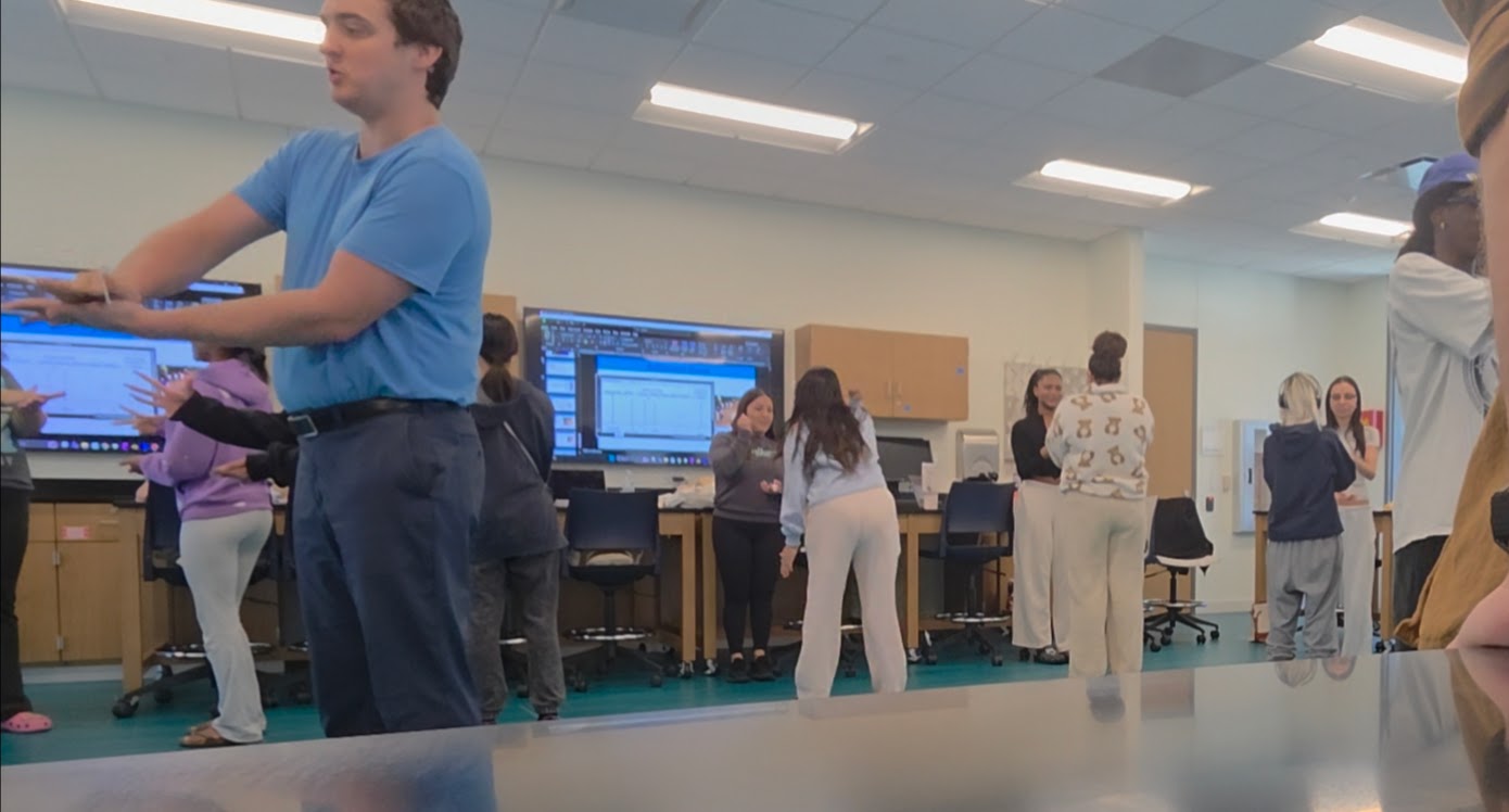
This simulator is inspired by a classroom activity often called Boltzmann Bucks, where students stand in concentric circles playing rock-paper-scissors, swapping energy tokens and then moving on to a new partner to repeat the process. Over time, the class naturally develops an uneven distribution of energy, reresenting the 2nd Law of Thermodynamics. Even though the rules are simple and the exchanges are random, a predictable statistical pattern emerges. Activities like this help students understand one of the central ideas of statistical mechanics: equilibrium does not mean equal distribution. Instead, equilibrium corresponds to the distribution that can occur in the greatest number of microscopic ways. The idea for this simulator is based on classroom activities described by Ben Meacham and earlier work in chemical education exploring token-exchange models of entropy and multiplicity.

Students participating in a classroom exchange activity. Screenshot of the Boltzmann Game simulator in progress.

How to Use the Simulator

1
Choose Settings
Set the number of students and rounds.
2
Start the Run
Click Start to begin the simulation.
3
Watch the Exchange
Observe energy transfers in the concentric rings.
4
Read the Results
Use the plots and tables to interpret the evolving distribution.
Simulator
Parameters
1.00x

Increasing the number of students and rounds produces smoother statistical behavior and results that more closely match theoretical predictions.

  • Maximum students: 1000
  • Maximum rounds: 1,000,000
Inner ring (gradient reds)
Outer ring
Relative Probability Scatter
(click to enlarge)
No fit applied.
Table 1 Style Distribution
Results

This panel summarizes how the current macrostate compares to the most probable equilibrium-like region of the system.

Relative Probability
\(P = 0\)
How close the current macrostate is to the most probable one.
Initial \(\ln W\)
\(\ln W = 0\)
The simulation starting point for comparison.
Equilibrium \(\ln W\)
\(\ln W = \text{pending}\)
The long-term plateau once the run is complete.
Higher values of \(P\) and \(\ln W\) usually indicate the system is spending more time in statistically common, equilibrium-like macrostates. Small fluctuations are normal.

Point of the Game

This simulation models a closed system where a fixed amount of energy is exchanged randomly between students. No energy is created or destroyed. Instead, energy moves from one student to another during each round of the game. This makes the activity a simple model of how microscopic randomness can lead to predictable large-scale statistical behavior.

At the beginning of the simulation, every student starts with exactly 1 unit of energy. Students are arranged on two concentric rings and paired by alignment each round. Each pair plays a simulated rock–paper–scissors interaction which determines whether energy moves between them.

How one round works

  • Pairing: An inner-ring student is paired with the aligned outer-ring student.
  • Random outcome: Each pair receives a random rock-paper-scissors result.
  • Win: If one student wins and the loser has at least 1 energy, 1 unit transfers from loser to winner.
  • Tie: If the result is a tie, no energy changes hands.
  • No change: If a student loses but has 0 energy, nothing transfers.
  • Rotation: After the round, the inner ring rotates so new pairs form for the next round.

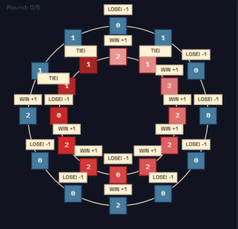
Example: Mid-round screenshot

Mid-round screenshot of the Boltzmann Game showing pairs, outcomes, and energy transfers.

A mid-round view of the simulation. Some pairs result in energy transfer, some tie, and some produce no change because the losing student has zero energy.

The exact assignment of energy to each individual student is called a microstate. However, we can also summarize the system using a broader description such as "8 students have 0 energy, 4 have 1 energy, 2 have 2 energy," and so on. That summary description is called a macrostate.

The key idea of the simulation is that some macrostates can occur in far more ways than others. Over time, the system naturally spends most of its time in macrostates that can be realized by many different microscopic arrangements. These highly realizable states correspond to what we call equilibrium.

Variable Definitions

Variable Definitions

Symbol Meaning Plain-language interpretation
\(N\)Total number of studentsThe number of participants (particles) in the system.
\(E\)Total energyThe fixed amount of energy shared among students. Here \(E=N\).
\(k\)Energy levelA possible energy value a student can have (0, 1, 2, 3...).
\(n_k\)Number of students with energy \(k\)How many students currently sit at that energy level.
\(W\)MultiplicityThe number of microstates corresponding to the macrostate.
\(W_{max}\)Maximum multiplicityThe largest possible value of \(W\).
\(\ln W\)Log multiplicityUsed because \(W\) becomes extremely large.
\(S\)EntropyA measure of how many microscopic arrangements are possible.
\(P_{rel}\)Relative probabilityHow close the current macrostate is to the most probable one.
\(t\)Round numberThe time-like index for simulation progress.
\(T\)Number of rounds in histogram averagingHow many rounds contribute to the averaged histogram.
\(y_{\infty}\)Equilibrium plateauThe long-term value approached by the running average near equilibrium.
\(A\)Initial offsetThe starting difference between the system and equilibrium.
\(\tau\)Relaxation timeThe timescale for approaching equilibrium.

Calculations

Each round produces a macrostate describing how many students occupy each energy level. Instead of tracking which specific student has which energy, we count how many students have 0 energy, how many have 1 energy, how many have 2 energy, and so on.

The formulas below allow the simulation to measure how typical the current macrostate is and how the system evolves toward equilibrium over time.

\[ \sum_k n_k = N,\quad \sum_k k n_k = E \]

These equations define a valid macrostate. The first says the total number of students must remain constant. The second says that when all student energies are added together, the total energy must remain fixed.

Microstates and Entropy

\[ W = \frac{N!}{\prod_k n_k!} \]

This equation counts how many distinct microscopic arrangements produce the same macrostate. A macrostate with a larger value of \(W\) can occur in more ways and is therefore statistically more likely.

\[ S \propto \ln W \]

Entropy is proportional to the logarithm of the multiplicity. The logarithm is used because the number of microstates becomes extremely large very quickly.

Relative Probability

\[ P_{rel} = \frac{W}{W_{max}} \]

This compares the multiplicity of the current macrostate to the multiplicity of the most probable macrostate. Values close to 1 indicate the system is near equilibrium.

Running Average

\[ \overline{\ln W}_n = \frac{1}{n}\sum_{i=1}^n \ln W_i \]

Individual rounds fluctuate significantly, so the running average smooths out noise and reveals the long-term trend toward equilibrium.

Histogram Averaging

\[ \overline{n_k} = \frac{1}{T}\sum_{t=1}^T n_k(t) \]

The histogram can display either the current distribution or a time-averaged distribution. Averaging produces a more stable comparison with theoretical predictions.

Interpreting Results

The most probable macrostate is the distribution that maximizes the multiplicity \(W\). For systems with mean energy near 1, the expected equilibrium-like distribution follows:

\[ n_k \approx \frac{N}{2^{k+1}} \]
Energy Level \(k\) Typical Count (N=24) Interpretation
0≈12Roughly half the students have no energy.
1≈6A smaller group holds 1 unit.
2≈3Fewer students accumulate 2 units.
3≈1-2High-energy students are uncommon.
4+RareVery high energy is possible but unlikely.

Equilibrium does not mean equal sharing of energy. Instead, it means the system fluctuates around macrostates that can occur in the greatest number of ways.

  • If \(\ln W\) levels off, the system is near equilibrium.
  • If \(P_{rel}\) fluctuates mostly near 1, the system frequently visits near-equilibrium macrostates.
  • If the histogram matches the theoretical curve, the energy distribution is behaving as expected.
Plot Guide and Fits

The simulator can display several different views of the same underlying process. Some plots show how typical the current macrostate is, some show how the system approaches equilibrium over time, and some compare the observed energy distribution to the theoretical expectation.

Relative Probability

Relative probability compares the current macrostate to the most probable one on a normalized scale. Values near 1 correspond to very typical macrostates, while smaller values correspond to rarer configurations that can be realized in fewer microscopic ways.

\[ P_{rel} = \frac{W}{W_{max}} \]

In a finite random system, the curve usually does not climb smoothly to 1 and stay there. Instead, it typically rises away from a low-probability start and then fluctuates within a higher-probability band once the system has settled into equilibrium-like behavior.

What to look for: An early rise or drift followed by noisy fluctuations in a stable band is normal. Brief dips do not mean the system has stopped behaving correctly.
Illustrative example \((N = 24)\)
Example only: a typical relative-probability trend rises from a low-probability start and then fluctuates in a stable band.

Entropy Scatter

Larger \(\ln W\) means the current macrostate can be realized in more microscopic ways and is therefore statistically more common. The raw scatter points represent individual rounds and can jump around substantially, while the running average reveals the long-term direction more clearly.

\[ S \propto \ln W \]

Even after the system reaches equilibrium-like behavior, individual rounds still fluctuate. What matters is the broad statistical level around which those rounds cluster.

What to look for: The cloud of points may remain noisy even after equilibrium is reached, but the running average should level into a relatively stable plateau region.
Illustrative example \((N = 24)\)
Example only: individual entropy values fluctuate strongly, while the running average settles toward a plateau.

Equilibrium Fit

The equilibrium fit is applied to the running-average entropy curve, not to every individual point. It provides a compact summary of the large-scale approach to equilibrium rather than trying to reproduce every short-term fluctuation.

\[ y(t) = y_{\infty} - A e^{-t/\tau} \]

Here \(y_{\infty}\) is the long-term plateau, \(A\) is how far below that plateau the system starts, and \(\tau\) is the relaxation timescale describing how quickly the average approaches equilibrium.

What to look for: A reasonable fit should track the broad shape of the running-average entropy curve without matching every fluctuation. The fit is most useful as a summary of trend rather than a perfect prediction.
Illustrative example \((N = 24)\)
Example only: the dashed fit captures the overall exponential approach, while the running average retains mild noise.

Energy Histogram

The bars show how many students currently occupy each energy level \(k\), while the theoretical line shows the expected equilibrium-like distribution for a system with mean energy 1.

\[ n_k = N\left(\frac{1}{2}\right)^{k+1} \]

For \(N=24\), a typical equilibrium-like shape means many students at 0 or 1 energy, fewer at 2, fewer still at 3, and only rare cases at higher energies.

What to look for: The current-round histogram may look jagged and irregular, especially early in the run, but the time-averaged histogram should settle into a smoother decaying shape that more closely follows the theoretical line.
Illustrative example \((N = 24)\)
Example only: bars wobble around an equilibrium-like decaying distribution, with the theoretical line shown as a reference.
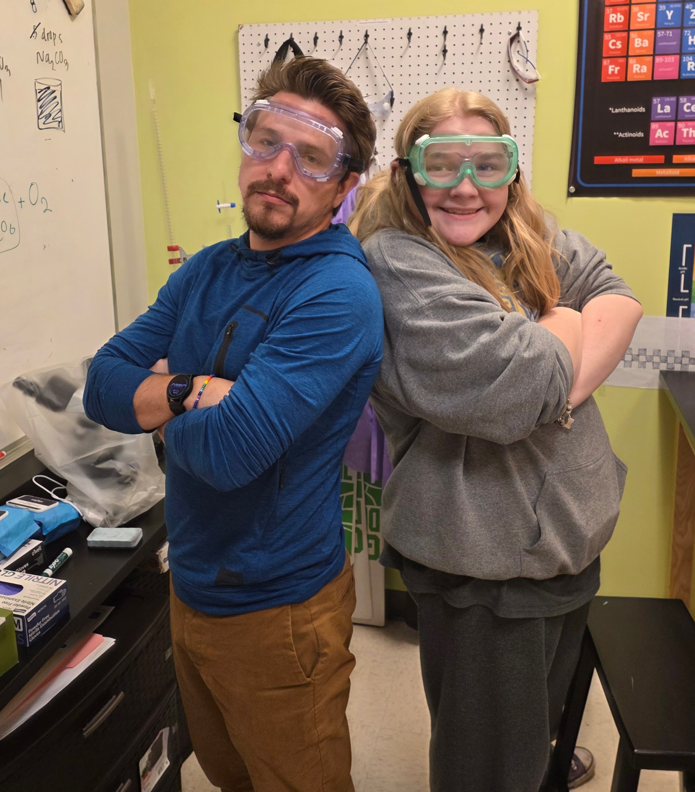
Portrait of David Mueller.
About the Creator

David Mueller

David Mueller, M.S. Physics, 2019. Teacher of High School Math and Physics at Fusion Academy and Instructor of Physics at Tarrant County College.

Runs the YouTube channel Meromorphic. For inquiries, contact dmueller787@gmail.com.

M.S. Physics, 2019 Fusion Academy Tarrant County College YouTube: Meromorphic dmueller787@gmail.com